Run INSPIRE on the brain datasets generated by Slide-seq V2 and MERFISH
In this tutorial, we show INSPIRE’s capability of integrating and interpreting ST brain datasets across different technologies (Slide-seq V2 and MERFISH). The cross-technology integration enables multiple downstream analysis to facilitate deep biological insights.
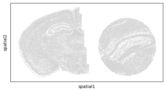
The mouse brain slice profiled by Slide-seq V2 is publicly available at https://singlecell.broadinstitute.org/single_cell.
The mouse brain slice profiled by MERFISH is publicly available at https://doi.brainimagelibrary.org/doi/10.35077/act-bag.
Import packages
[1]:
import pandas as pd
import numpy as np
import scanpy as sc
import anndata as ad
import umap
import os
import matplotlib.pyplot as plt
import matplotlib as mpl
from matplotlib.cm import get_cmap
from matplotlib.lines import Line2D

import INSPIRE

import warnings
warnings.filterwarnings("ignore")
Load data
[2]:
print("Load Slide-seq V2 data...")
data_dir = "/gpfs/gibbs/project/zhao/jz874/jiazhao/reference-free_spatial-integration/data/SlideseqV2_mouse_hippocampus"
adata_slideseqv2 = sc.read_h5ad(data_dir+"/adata_slideseqv2_Puck_200115_08.h5ad")
adata_slideseqv2.var_names_make_unique()
Load Slide-seq V2 data...
[3]:
print("Load MERFISH data...")
data_dir = "/gpfs/gibbs/project/zhao/jz874/jiazhao/reference-free_spatial-integration/data/MERFISH_mouse_hippocampus"
adata_merfish = sc.read_h5ad(data_dir + "/raw_counts_mouse1_coronal.h5ad")
adata_merfish = adata_merfish[adata_merfish.obs["slice_id"] == "co1_slice37", :]
adata_merfish.var_names_make_unique()
adata_merfish.obsm["spatial"] = np.array(adata_merfish.obs[["center_x","center_y"]].values)
adata_merfish.obsm["spatial"][:,1] = -adata_merfish.obsm["spatial"][:,1]
Load MERFISH data...
[4]:
adata_st_list = [adata_merfish, adata_slideseqv2]
Data preprocessing
[5]:
adata_st_list, adata_full = INSPIRE.utils.preprocess(adata_st_list=adata_st_list,
                                                     num_hvgs=1000,
                                                     min_genes_qc=6,
                                                     min_cells_qc=6,
                                                     spot_size=30,
                                                     limit_num_genes=True)
Get shared genes among all datasets...
Find 1077 shared genes among datasets.
Finding highly variable genes...
shape of adata 0 before quality control:  (44959, 1077)
shape of adata 0 after quality control:  (44950, 1077)
shape of adata 1 before quality control:  (53208, 1077)
shape of adata 1 after quality control:  (29866, 1019)
Find 936 shared highly variable genes among datasets.
Concatenate datasets as a full anndata for better visualization...
Store counts and library sizes for Poisson modeling...
Normalize data...
Build spatial graph and prepare node features for LGCN
[6]:
adata_st_list = INSPIRE.utils.build_graph_LGCN(adata_st_list=adata_st_list,
                                               rad_cutoff_list=[100,100])
Start building graphs...
Build graphs and prepare node features for LGCN networks
Radius for graph connection is 100.0000.
59.4303 neighbors per cell on average.
Node features for slice 0 : (44950, 1872)
Radius for graph connection is 100.0000.
55.3459 neighbors per cell on average.
Node features for slice 1 : (29866, 1872)
Run INSPIRE model
[7]:
model = INSPIRE.model.Model_LGCN(adata_st_list=adata_st_list,
                                 n_spatial_factors=40,
                                 n_training_steps=20000,
                                 batch_size=2048,
                                 different_platforms=True
                                )
[8]:
model.train(adata_st_list)
0%| | 3/20000 [00:00<44:40, 7.46it/s]
Step: 0, d_loss: 1.3804, Loss: 1107.8776, recon_loss: 364.2183, fe_loss: 33.9514, geom_loss: 152.0855, beta_loss: 706.0208, gan_loss: 0.6454
3%|▎ | 503/20000 [00:39<25:53, 12.55it/s]
Step: 500, d_loss: 0.4739, Loss: 1062.8374, recon_loss: 327.0807, fe_loss: 26.8601, geom_loss: 212.4773, beta_loss: 701.3384, gan_loss: 3.3085
5%|▌ | 1003/20000 [01:19<25:06, 12.61it/s]
Step: 1000, d_loss: 0.3885, Loss: 1034.2128, recon_loss: 297.9872, fe_loss: 26.2441, geom_loss: 226.5229, beta_loss: 701.4506, gan_loss: 4.0004
8%|▊ | 1503/20000 [01:59<24:22, 12.64it/s]
Step: 1500, d_loss: 0.4212, Loss: 1013.1816, recon_loss: 277.0578, fe_loss: 26.0369, geom_loss: 208.2087, beta_loss: 701.9286, gan_loss: 3.9940
10%|█ | 2003/20000 [02:38<23:56, 12.53it/s]
Step: 2000, d_loss: 0.4306, Loss: 991.0729, recon_loss: 255.2527, fe_loss: 25.7833, geom_loss: 214.4679, beta_loss: 701.8830, gan_loss: 3.8646
13%|█▎ | 2503/20000 [03:18<23:10, 12.58it/s]
Step: 2500, d_loss: 0.5530, Loss: 977.2664, recon_loss: 241.8146, fe_loss: 25.6681, geom_loss: 198.2184, beta_loss: 701.9707, gan_loss: 3.8487
15%|█▌ | 3003/20000 [03:57<22:26, 12.63it/s]
Step: 3000, d_loss: 0.4567, Loss: 959.5751, recon_loss: 225.1785, fe_loss: 25.2786, geom_loss: 188.4720, beta_loss: 701.9492, gan_loss: 3.3995
18%|█▊ | 3503/20000 [04:37<21:43, 12.65it/s]
Step: 3500, d_loss: 0.4580, Loss: 953.8770, recon_loss: 219.9923, fe_loss: 25.2972, geom_loss: 177.6109, beta_loss: 701.8467, gan_loss: 3.1885
20%|██ | 4003/20000 [05:16<21:11, 12.59it/s]
Step: 4000, d_loss: 0.4336, Loss: 944.5686, recon_loss: 210.9358, fe_loss: 25.2467, geom_loss: 172.2353, beta_loss: 701.8006, gan_loss: 3.1408
23%|██▎ | 4503/20000 [05:56<20:23, 12.66it/s]
Step: 4500, d_loss: 0.4527, Loss: 937.1896, recon_loss: 203.9106, fe_loss: 25.0024, geom_loss: 167.1406, beta_loss: 702.0719, gan_loss: 2.8620
25%|██▌ | 5003/20000 [06:35<19:44, 12.66it/s]
Step: 5000, d_loss: 0.4972, Loss: 937.3575, recon_loss: 204.3245, fe_loss: 25.0842, geom_loss: 162.6318, beta_loss: 701.7872, gan_loss: 2.9091
28%|██▊ | 5503/20000 [07:15<19:10, 12.60it/s]
Step: 5500, d_loss: 0.5321, Loss: 934.3118, recon_loss: 201.5955, fe_loss: 24.8613, geom_loss: 158.4373, beta_loss: 701.6425, gan_loss: 3.0438
30%|███ | 6003/20000 [07:54<18:33, 12.57it/s]
Step: 6000, d_loss: 0.4736, Loss: 927.1862, recon_loss: 195.0019, fe_loss: 24.7317, geom_loss: 154.3978, beta_loss: 701.5516, gan_loss: 2.8130
33%|███▎ | 6503/20000 [08:34<17:56, 12.54it/s]
Step: 6500, d_loss: 0.4030, Loss: 931.9471, recon_loss: 198.3225, fe_loss: 25.3106, geom_loss: 167.3774, beta_loss: 701.6801, gan_loss: 3.2864
35%|███▌ | 7003/20000 [09:14<17:08, 12.64it/s]
Step: 7000, d_loss: 0.2965, Loss: 932.3434, recon_loss: 197.4599, fe_loss: 25.2167, geom_loss: 182.9161, beta_loss: 701.7018, gan_loss: 4.3067
38%|███▊ | 7503/20000 [09:53<16:32, 12.59it/s]
Step: 7500, d_loss: 0.2778, Loss: 927.1822, recon_loss: 192.9050, fe_loss: 25.0668, geom_loss: 177.7019, beta_loss: 701.5798, gan_loss: 4.0767
40%|████ | 8003/20000 [10:33<15:55, 12.56it/s]
Step: 8000, d_loss: 0.2667, Loss: 925.1646, recon_loss: 190.6947, fe_loss: 25.0511, geom_loss: 174.0815, beta_loss: 701.7958, gan_loss: 4.1413
43%|████▎ | 8503/20000 [11:12<15:10, 12.63it/s]
Step: 8500, d_loss: 0.3204, Loss: 927.0892, recon_loss: 192.6733, fe_loss: 24.9504, geom_loss: 183.8102, beta_loss: 701.7314, gan_loss: 4.0579
45%|████▌ | 9003/20000 [11:52<14:28, 12.66it/s]
Step: 9000, d_loss: 0.5917, Loss: 924.4792, recon_loss: 190.6605, fe_loss: 24.9616, geom_loss: 194.0464, beta_loss: 701.6375, gan_loss: 3.3386
48%|████▊ | 9503/20000 [12:31<13:50, 12.64it/s]
Step: 9500, d_loss: 0.4401, Loss: 919.8731, recon_loss: 185.7394, fe_loss: 24.8804, geom_loss: 197.0424, beta_loss: 701.9235, gan_loss: 3.3890
50%|█████ | 10003/20000 [13:11<13:15, 12.56it/s]
Step: 10000, d_loss: 0.4786, Loss: 924.5259, recon_loss: 189.7460, fe_loss: 25.0542, geom_loss: 202.3312, beta_loss: 701.6459, gan_loss: 4.0332
53%|█████▎ | 10503/20000 [13:50<12:34, 12.59it/s]
Step: 10500, d_loss: 1.0833, Loss: 925.1063, recon_loss: 190.3775, fe_loss: 24.9870, geom_loss: 195.0566, beta_loss: 701.4221, gan_loss: 4.4186
55%|█████▌ | 11003/20000 [14:30<11:53, 12.62it/s]
Step: 11000, d_loss: 0.6127, Loss: 925.0593, recon_loss: 191.4999, fe_loss: 25.1023, geom_loss: 175.7487, beta_loss: 701.7168, gan_loss: 3.2253
58%|█████▊ | 11503/20000 [15:09<11:13, 12.62it/s]
Step: 11500, d_loss: 0.5606, Loss: 920.9508, recon_loss: 186.8466, fe_loss: 25.0311, geom_loss: 181.0251, beta_loss: 701.9043, gan_loss: 3.5483
60%|██████ | 12003/20000 [15:49<10:33, 12.62it/s]
Step: 12000, d_loss: 0.5772, Loss: 919.0579, recon_loss: 186.0927, fe_loss: 25.0327, geom_loss: 171.7448, beta_loss: 701.7373, gan_loss: 2.7602
63%|██████▎ | 12503/20000 [16:28<09:53, 12.62it/s]
Step: 12500, d_loss: 0.5493, Loss: 922.0925, recon_loss: 188.3122, fe_loss: 25.1438, geom_loss: 172.0260, beta_loss: 701.8330, gan_loss: 3.3629
65%|██████▌ | 13003/20000 [17:08<09:11, 12.69it/s]
Step: 13000, d_loss: 0.5241, Loss: 917.9173, recon_loss: 184.3802, fe_loss: 24.8213, geom_loss: 204.9407, beta_loss: 701.5182, gan_loss: 3.0988
68%|██████▊ | 13503/20000 [17:47<08:36, 12.57it/s]
Step: 13500, d_loss: 0.6190, Loss: 917.5731, recon_loss: 184.0115, fe_loss: 24.8391, geom_loss: 199.5222, beta_loss: 701.6268, gan_loss: 3.1053
70%|███████ | 14003/20000 [18:27<07:55, 12.61it/s]
Step: 14000, d_loss: 0.5522, Loss: 920.2089, recon_loss: 186.5747, fe_loss: 25.0187, geom_loss: 182.4173, beta_loss: 701.6837, gan_loss: 3.2834
73%|███████▎ | 14503/20000 [19:06<07:13, 12.67it/s]
Step: 14500, d_loss: 0.5803, Loss: 917.8388, recon_loss: 184.8993, fe_loss: 24.7555, geom_loss: 176.9848, beta_loss: 701.6060, gan_loss: 3.0384
75%|███████▌ | 15003/20000 [19:46<06:34, 12.65it/s]
Step: 15000, d_loss: 0.5058, Loss: 918.8309, recon_loss: 185.4706, fe_loss: 24.9070, geom_loss: 170.9167, beta_loss: 701.6613, gan_loss: 3.3737
78%|███████▊ | 15503/20000 [20:25<05:56, 12.60it/s]
Step: 15500, d_loss: 0.5948, Loss: 916.8358, recon_loss: 183.5508, fe_loss: 24.8522, geom_loss: 160.7567, beta_loss: 701.7112, gan_loss: 3.5064
80%|████████ | 16003/20000 [21:05<05:18, 12.56it/s]
Step: 16000, d_loss: 0.5975, Loss: 914.3005, recon_loss: 181.9464, fe_loss: 24.7472, geom_loss: 172.2131, beta_loss: 701.3987, gan_loss: 2.7639
83%|████████▎ | 16503/20000 [21:44<04:37, 12.61it/s]
Step: 16500, d_loss: 0.6016, Loss: 915.2278, recon_loss: 182.7234, fe_loss: 24.7153, geom_loss: 164.6563, beta_loss: 701.5428, gan_loss: 2.9531
85%|████████▌ | 17003/20000 [22:24<03:57, 12.61it/s]
Step: 17000, d_loss: 0.5983, Loss: 912.9772, recon_loss: 181.2617, fe_loss: 24.7501, geom_loss: 154.2357, beta_loss: 701.4165, gan_loss: 2.4642
88%|████████▊ | 17503/20000 [23:04<03:18, 12.56it/s]
Step: 17500, d_loss: 0.5978, Loss: 916.6935, recon_loss: 184.0978, fe_loss: 24.8059, geom_loss: 153.6965, beta_loss: 701.6282, gan_loss: 3.0878
90%|█████████ | 18003/20000 [23:43<02:38, 12.63it/s]
Step: 18000, d_loss: 0.5956, Loss: 915.1566, recon_loss: 182.7483, fe_loss: 24.7924, geom_loss: 144.8719, beta_loss: 701.5306, gan_loss: 3.1877
93%|█████████▎| 18503/20000 [24:23<01:59, 12.54it/s]
Step: 18500, d_loss: 0.6158, Loss: 912.2043, recon_loss: 180.8354, fe_loss: 24.7071, geom_loss: 152.1731, beta_loss: 701.4999, gan_loss: 2.1185
95%|█████████▌| 19003/20000 [25:02<01:18, 12.64it/s]
Step: 19000, d_loss: 0.6072, Loss: 915.9505, recon_loss: 183.3734, fe_loss: 24.8276, geom_loss: 152.4524, beta_loss: 701.6520, gan_loss: 3.0484
98%|█████████▊| 19503/20000 [25:42<00:39, 12.58it/s]
Step: 19500, d_loss: 0.5961, Loss: 914.7076, recon_loss: 182.7415, fe_loss: 24.6228, geom_loss: 145.4396, beta_loss: 701.5344, gan_loss: 2.9001
100%|██████████| 20000/20000 [26:21<00:00, 12.65it/s]
Access spot representations, proportions of spatial factors in spots, and gene loading matrix
[9]:
adata_full, basis_df = model.eval(adata_st_list, adata_full)
basis = np.array(basis_df.values)
Add cell/spot proportions of spatial factors into adata_full.obs...
Add cell/spot latent representations into adata_full.obsm['latent']...
Gene loading matrix is saved as basis.
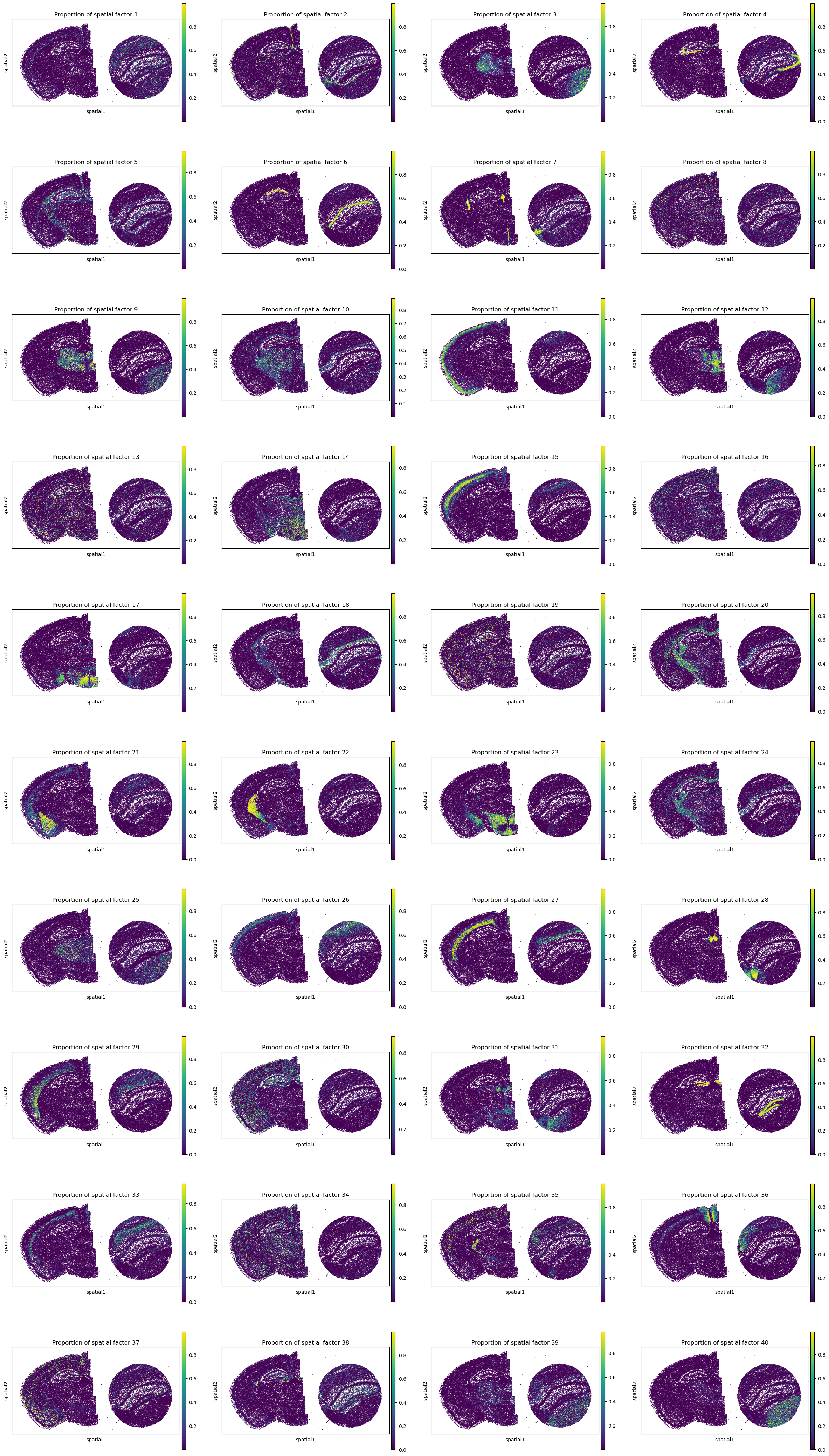
Spatial distributions of spatial factors in tissues
[10]:
sc.pl.spatial(adata_full, color=["Proportion of spatial factor "+str(i+1) for i in range(40)], spot_size=40.)
Spot representations and spatial domain identification
[11]:
reducer = umap.UMAP(n_neighbors=30,
                    n_components=2,
                    metric="correlation",
                    n_epochs=None,
                    learning_rate=1.0,
                    min_dist=0.3,
                    spread=1.0,
                    set_op_mix_ratio=1.0,
                    local_connectivity=1,
                    repulsion_strength=1,
                    negative_sample_rate=5,
                    a=None,
                    b=None,
                    random_state=1234,
                    metric_kwds=None,
                    angular_rp_forest=False,
                    verbose=True)
embedding = reducer.fit_transform(adata_full.obsm['latent'])
adata_full.obsm["X_umap"] = embedding
adata_full.obs["slice"] = adata_full.obs["slice"].values.astype(str)
UMAP(angular_rp_forest=True, local_connectivity=1, metric='correlation', min_dist=0.3, n_neighbors=30, random_state=1234, repulsion_strength=1, verbose=True)
Fri Aug 23 17:03:28 2024 Construct fuzzy simplicial set
Fri Aug 23 17:03:28 2024 Finding Nearest Neighbors
Fri Aug 23 17:03:28 2024 Building RP forest with 19 trees
Fri Aug 23 17:03:30 2024 NN descent for 16 iterations
         1  /  16
         2  /  16
         3  /  16
        Stopping threshold met -- exiting after 3 iterations
Fri Aug 23 17:03:43 2024 Finished Nearest Neighbor Search
Fri Aug 23 17:03:50 2024 Construct embedding
        completed  0  /  200 epochs
        completed  20  /  200 epochs
        completed  40  /  200 epochs
        completed  60  /  200 epochs
        completed  80  /  200 epochs
        completed  100  /  200 epochs
        completed  120  /  200 epochs
        completed  140  /  200 epochs
        completed  160  /  200 epochs
        completed  180  /  200 epochs
Fri Aug 23 17:05:15 2024 Finished embedding
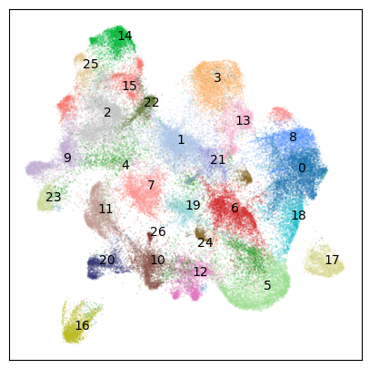
[12]:
# perform spatial domain identification task by clustering on cell representations.
sc.pp.neighbors(adata_full, use_rep="latent")
sc.tl.louvain(adata_full, resolution=1.2)
Visualization of cell representations
[13]:
adata = adata_full

size = 0.02
umap = adata.obsm["X_umap"]
n_cells = umap.shape[0]
np.random.seed(1234)
order = np.arange(n_cells)
np.random.shuffle(order)

adata.obs["slice_color"] = ""
adata.obs["slice_color"][adata.obs["slice"].values.astype(str) == str(0)] = "tab:blue"
adata.obs["slice_color"][adata.obs["slice"].values.astype(str) == str(1)] = "tab:orange"

f = plt.figure(figsize=(5,5))

ax3 = f.add_subplot(1,1,1)
scatter2 = ax3.scatter(umap[order, 0], umap[order, 1], s=size, c=adata.obs["slice_color"][order], rasterized=True, marker='o')
ax3.tick_params(axis='both',bottom=False, top=False, left=False, right=False, labelleft=False, labelbottom=False, grid_alpha=0)

legend_elements_slice = [Line2D([0], [0], marker='o', color="w", label='MERFISH', markerfacecolor="tab:blue", markersize=10),
                         Line2D([0], [0], marker='o', color="w", label='Slide-seq V2', markerfacecolor="tab:orange", markersize=10)]
ax3.legend(handles=legend_elements_slice, loc="upper left", bbox_to_anchor=(1, 1.), frameon=False,
           markerscale=.8, fontsize=10, handletextpad=0., ncol=1)

f.subplots_adjust(hspace=0.02, wspace=0.1)
plt.show()

[14]:
# setup colors

rgb_10 = [i for i in get_cmap('Set3').colors]
rgb_20 = [i for i in get_cmap('tab20').colors]
rgb_20b = [i for i in get_cmap('tab20b').colors]
rgb_dark2 = [i for i in get_cmap('Dark2').colors]
rgb_pst1 = [i for i in get_cmap('Pastel1').colors]
rgb_acc = [i for i in get_cmap('Accent').colors]
rgb2hex_10 = [mpl.colors.rgb2hex(color) for color in rgb_10]
rgb2hex_20 = [mpl.colors.rgb2hex(color) for color in rgb_20]
rgb2hex_20b = [mpl.colors.rgb2hex(color) for color in rgb_20b]
rgb2hex_20b_new = [rgb2hex_20b[i] for i in [0, 3, 4, 7, 8, 11, 12, 15, 16, 19]]
rgb2hex_dark2 = [mpl.colors.rgb2hex(color) for color in rgb_dark2]
rgb2hex_pst1 = [mpl.colors.rgb2hex(color) for color in rgb_pst1]
rgb2hex_acc = [mpl.colors.rgb2hex(color) for color in rgb_acc]
rgb2hex = rgb2hex_20 + rgb2hex_20b_new + rgb2hex_dark2 + rgb2hex_pst1 + rgb2hex_acc
colors = rgb2hex
adata.obs["louvain_color"] = ""
for i in range(len(set(adata.obs["louvain"].values.astype(str)))):
    adata.obs["louvain_color"][adata.obs["louvain"].values.astype(str) == str(i)] = colors[i]

adata.obs["louvain_color"][adata.obs["louvain"].values.astype(str) == str(8)] = "#619CFF"
adata.obs["louvain_color"][adata.obs["louvain"].values.astype(str) == str(14)] = "#00BA38"
adata.obs["louvain_color"][adata.obs["louvain"].values.astype(str) == str(15)] = "#F8766D"
adata.obs["louvain_color"][adata.obs["louvain"].values.astype(str) == str(2)] = rgb2hex[15]
[15]:
size = 0.01
umap = adata.obsm["X_umap"]
n_cells = umap.shape[0]
np.random.seed(1234)
order = np.arange(n_cells)
np.random.shuffle(order)

f = plt.figure(figsize=(5,5))

ax3 = f.add_subplot(1,1,1)
scatter2 = ax3.scatter(umap[order, 0], umap[order, 1], s=size, c=adata.obs["louvain_color"][order], rasterized=True, marker='o')
ax3.tick_params(axis='both',bottom=False, top=False, left=False, right=False, labelleft=False, labelbottom=False, grid_alpha=0)

for i in range(len(set(adata.obs["louvain"].values.astype(str)))):
    coor_tmp = umap[adata.obs["louvain"].values.astype(str) == str(i), :]
    coor_xy = np.median(coor_tmp, axis=0)
    if i == 24:
        coor_xy[0] = 6.5
        coor_xy[1] = 5.5
        ax3.annotate(str(i), coor_xy)
    elif i == 4:
        coor_xy[0] = 2
        coor_xy[1] = 9.5
        ax3.annotate(str(i), coor_xy)
    else:
        ax3.annotate(str(i), coor_xy)

f.subplots_adjust(hspace=0.02, wspace=0.1)
plt.show()
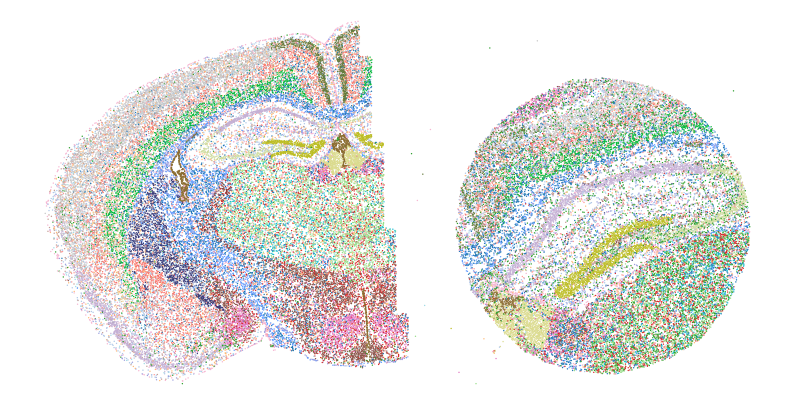
Visualization of spatial domain identification result
[16]:
size = 1.
n_louvain = len(set(adata.obs["louvain"]))
f = plt.figure(figsize=(10,5))
ax = f.add_subplot(1,1,1)
ax.axis('equal')
colors = rgb2hex
ax.scatter(adata.obsm["spatial"][:, 0],
           -adata.obsm["spatial"][:, 1],
           s=size, facecolors=adata.obs["louvain_color"], edgecolors='none', rasterized=True)
ax.set_axis_off()
f.subplots_adjust(hspace=0.02, wspace=0.1)
plt.show()
Save results
[17]:
### Save results
res_path = "Results/INSPIRE_diff_tech_brain"
adata_full.write(res_path + "/adata_inspire.h5ad")
basis_df.to_csv(res_path + "/basis_df_inspire.csv")