Run INSPIRE on multiple mouse embryo slices for 3D reconstruction
In this tutorial, we show INSPIRE’s ability to build 3D model of mouse embryo by integrating multiple 2D slices.
The mouse embryo data are publicly available at https://db.cngb.org/stomics/mosta/download/.
Import packages
[1]:
import pandas as pd
import numpy as np
import scanpy as sc
import anndata as ad
import umap
import os
import scipy.sparse
import matplotlib.pyplot as plt
from matplotlib.cm import get_cmap
import matplotlib as mpl
from matplotlib.lines import Line2D

import INSPIRE

import warnings
warnings.filterwarnings("ignore")
Data preprocessing
Each ST slice contained a large number of spatial spots. For efficiency, we preprocessed each slice respectively.
[ ]:
# slice_name = "E16.5_E2S8"

# # Load data
# print("load data", slice_name)
# data_dir = "data/Stereoseq_mouse_embryo"
# adata = sc.read_h5ad(os.path.join(data_dir, slice_name+".MOSTA.h5ad"))
# adata.X = adata.layers['count']
# adata.var_names_make_unique()
# adata.obs_names_make_unique()

# # Preprocess data
# INSPIRE.utils.calculate_node_features_LGCN(adata=adata,
#                                            slice_name=slice_name,
#                                            preprocessed_data_path="data/Stereoseq_mouse_embryo/preprocessed_data_3d",
#                                            min_genes_qc=50,
#                                            min_cells_qc=50,
#                                            rad_cutoff=1.6
#                                           )
The data after preprocessing are saved into preprocessed_data_path.
Load preprocessed data
[2]:
slice_name_list = ["E16.5_E2S8", "E16.5_E2S9", "E16.5_E2S10", "E16.5_E2S11", "E16.5_E2S12"]
preprocessed_data_path = "data/Stereoseq_mouse_embryo/preprocessed_data_3d"

adata_st_list, adata_full = INSPIRE.utils.prepare_inputs_LGCN(slice_name_list=slice_name_list,
                                                              preprocessed_data_path=preprocessed_data_path,
                                                              num_hvgs=8000,
                                                              spot_size=1.,
                                                              min_concat_dist=20)
Finding highly variable genes...
Load data E16.5_E2S8
Load data E16.5_E2S9
Load data E16.5_E2S10
Load data E16.5_E2S11
Load data E16.5_E2S12
Find 2966 shared highly variable genes among datasets.
Store counts and library sizes for Poisson modeling...
Normalize data...
Load data E16.5_E2S8
Load data E16.5_E2S9
Load data E16.5_E2S10
Load data E16.5_E2S11
Load data E16.5_E2S12
Load and prepare node features for LGCN...
Load node features E16.5_E2S8
Node features for slice 0 : (120676, 5932)
Load node features E16.5_E2S9
Node features for slice 1 : (129376, 5932)
Load node features E16.5_E2S10
Node features for slice 2 : (113759, 5932)
Load node features E16.5_E2S11
Node features for slice 3 : (109281, 5932)
Load node features E16.5_E2S12
Node features for slice 4 : (94289, 5932)
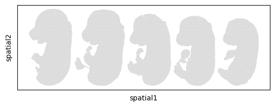
Prepare an adata containing full spot locations and slice labels for better visualization...
Run INSPIRE model
[3]:
model = INSPIRE.model.Model_LGCN(adata_st_list=adata_st_list,
                                 n_spatial_factors=60,
                                 n_training_steps=10000,
                                 batch_size=2048
                                )
[4]:
model.train(adata_st_list)
0%| | 1/10000 [00:02<6:50:37, 2.46s/it]
Step: 0, d_loss: 5.5533, Loss: 8648.1816, recon_loss: 7564.4771, fe_loss: 134.7938, geom_loss: 219.0089, beta_loss: 941.7137, gan_loss: 2.8164
5%|▌ | 501/10000 [03:54<1:13:30, 2.15it/s]
Step: 500, d_loss: 4.0936, Loss: 6799.6064, recon_loss: 5718.1675, fe_loss: 92.3857, geom_loss: 488.3807, beta_loss: 973.8798, gan_loss: 5.4058
10%|█ | 1001/10000 [07:45<1:10:00, 2.14it/s]
Step: 1000, d_loss: 3.8157, Loss: 5239.8032, recon_loss: 4104.0610, fe_loss: 91.3244, geom_loss: 454.3840, beta_loss: 1029.2563, gan_loss: 6.0736
15%|█▌ | 1501/10000 [11:34<1:05:46, 2.15it/s]
Step: 1500, d_loss: 3.7621, Loss: 3883.4690, recon_loss: 2714.4673, fe_loss: 91.1893, geom_loss: 440.1596, beta_loss: 1062.4374, gan_loss: 6.5719
20%|██ | 2001/10000 [15:25<1:02:37, 2.13it/s]
Step: 2000, d_loss: 3.7257, Loss: 2716.6931, recon_loss: 1540.6566, fe_loss: 90.9981, geom_loss: 465.1812, beta_loss: 1068.5623, gan_loss: 7.1727
25%|██▌ | 2501/10000 [19:16<58:26, 2.14it/s]
Step: 2500, d_loss: 3.9234, Loss: 1728.3782, recon_loss: 549.3525, fe_loss: 90.7758, geom_loss: 473.1777, beta_loss: 1072.6163, gan_loss: 6.1700
30%|███ | 3001/10000 [23:06<54:41, 2.13it/s]
Step: 3000, d_loss: 3.8576, Loss: 994.8348, recon_loss: -167.3379, fe_loss: 90.5017, geom_loss: 441.4391, beta_loss: 1057.0203, gan_loss: 5.8220
35%|███▌ | 3501/10000 [26:57<50:14, 2.16it/s]
Step: 3500, d_loss: 3.7828, Loss: 194.2820, recon_loss: -954.0574, fe_loss: 90.2834, geom_loss: 395.6738, beta_loss: 1044.0774, gan_loss: 6.0652
40%|████ | 4001/10000 [30:48<46:48, 2.14it/s]
Step: 4000, d_loss: 3.7493, Loss: -222.3103, recon_loss: -1349.1482, fe_loss: 90.0547, geom_loss: 369.0643, beta_loss: 1023.7653, gan_loss: 5.6368
45%|████▌ | 4501/10000 [34:39<42:36, 2.15it/s]
Step: 4500, d_loss: 3.7471, Loss: -341.5936, recon_loss: -1439.6331, fe_loss: 89.9799, geom_loss: 369.0586, beta_loss: 994.2235, gan_loss: 6.4548
50%|█████ | 5001/10000 [38:30<38:49, 2.15it/s]
Step: 5000, d_loss: 3.7183, Loss: -584.0801, recon_loss: -1671.0793, fe_loss: 90.0652, geom_loss: 369.7906, beta_loss: 983.2839, gan_loss: 6.2543
55%|█████▌ | 5501/10000 [42:21<35:02, 2.14it/s]
Step: 5500, d_loss: 3.8017, Loss: -694.8525, recon_loss: -1769.2306, fe_loss: 89.7439, geom_loss: 356.2195, beta_loss: 971.4628, gan_loss: 6.0470
60%|██████ | 6001/10000 [46:12<30:55, 2.15it/s]
Step: 6000, d_loss: 3.7726, Loss: -911.4283, recon_loss: -1978.8911, fe_loss: 89.8415, geom_loss: 361.3640, beta_loss: 964.2572, gan_loss: 6.1368
65%|██████▌ | 6501/10000 [50:04<27:16, 2.14it/s]
Step: 6500, d_loss: 3.7303, Loss: -780.4904, recon_loss: -1840.0757, fe_loss: 89.6845, geom_loss: 346.5454, beta_loss: 956.7856, gan_loss: 6.1842
70%|███████ | 7001/10000 [53:55<23:19, 2.14it/s]
Step: 7000, d_loss: 3.7897, Loss: -712.4079, recon_loss: -1766.1638, fe_loss: 89.7189, geom_loss: 322.4746, beta_loss: 951.6609, gan_loss: 5.9267
75%|███████▌ | 7501/10000 [57:46<19:19, 2.15it/s]
Step: 7500, d_loss: 3.7563, Loss: -879.4528, recon_loss: -1929.5426, fe_loss: 89.5975, geom_loss: 297.5077, beta_loss: 948.4641, gan_loss: 6.0780
80%|████████ | 8001/10000 [1:01:36<15:30, 2.15it/s]
Step: 8000, d_loss: 3.6589, Loss: -1095.2783, recon_loss: -2142.0918, fe_loss: 89.2430, geom_loss: 286.2124, beta_loss: 945.6093, gan_loss: 6.2370
85%|████████▌ | 8501/10000 [1:05:27<11:40, 2.14it/s]
Step: 8500, d_loss: 3.5608, Loss: -703.2833, recon_loss: -1747.6008, fe_loss: 89.3475, geom_loss: 278.3501, beta_loss: 942.7364, gan_loss: 6.6666
90%|█████████ | 9001/10000 [1:09:19<07:45, 2.15it/s]
Step: 9000, d_loss: 3.5137, Loss: -823.5667, recon_loss: -1866.2191, fe_loss: 89.4667, geom_loss: 268.2156, beta_loss: 941.1996, gan_loss: 6.6219
95%|█████████▌| 9501/10000 [1:13:10<03:51, 2.16it/s]
Step: 9500, d_loss: 3.6148, Loss: -1027.9996, recon_loss: -2068.3501, fe_loss: 89.2274, geom_loss: 255.3610, beta_loss: 939.6401, gan_loss: 6.3757
100%|██████████| 10000/10000 [1:17:00<00:00, 2.16it/s]
Access spot representations, proportions of spatial factors in spots, and gene loading matrix
We evaluate the spot representations and proportions of spatial factors in spots with minibatches.
[5]:
adata_full, basis_df = model.eval_minibatch(adata_st_list,
                                            adata_full,
                                            batch_size=10000
                                           )
Evaluate Z and beta using minibatch...
Evaluation for slice 0
Evaluation for slice 1
Evaluation for slice 2
Evaluation for slice 3
Evaluation for slice 4
[6]:
reducer = umap.UMAP(n_neighbors=30,
                    n_components=2,
                    metric="correlation",
                    n_epochs=None,
                    learning_rate=1.0,
                    min_dist=0.3,
                    spread=1.0,
                    set_op_mix_ratio=1.0,
                    local_connectivity=1,
                    repulsion_strength=1,
                    negative_sample_rate=5,
                    a=None,
                    b=None,
                    random_state=1234,
                    metric_kwds=None,
                    angular_rp_forest=False,
                    verbose=True)
embedding = reducer.fit_transform(adata_full.obsm['latent'])
adata_full.obsm["X_umap"] = embedding
adata_full.obs["slice_label"] = adata_full.obs["slice_label"].values.astype(str)
UMAP(angular_rp_forest=True, local_connectivity=1, metric='correlation', min_dist=0.3, n_neighbors=30, random_state=1234, repulsion_strength=1, verbose=True)
Sat Aug 24 14:15:28 2024 Construct fuzzy simplicial set
Sat Aug 24 14:15:28 2024 Finding Nearest Neighbors
Sat Aug 24 14:15:28 2024 Building RP forest with 43 trees
Sat Aug 24 14:15:34 2024 NN descent for 19 iterations
         1  /  19
         2  /  19
         3  /  19
        Stopping threshold met -- exiting after 3 iterations
Sat Aug 24 14:16:18 2024 Finished Nearest Neighbor Search
Sat Aug 24 14:16:26 2024 Construct embedding
        completed  0  /  200 epochs
        completed  20  /  200 epochs
        completed  40  /  200 epochs
        completed  60  /  200 epochs
        completed  80  /  200 epochs
        completed  100  /  200 epochs
        completed  120  /  200 epochs
        completed  140  /  200 epochs
        completed  160  /  200 epochs
        completed  180  /  200 epochs
Sat Aug 24 14:30:33 2024 Finished embedding
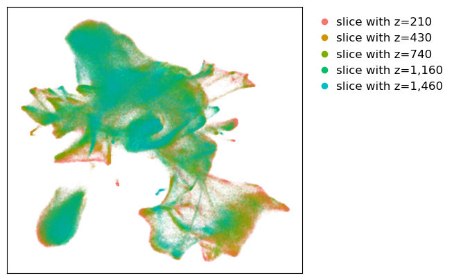
[7]:
adata = adata_full

size = 0.001
slice_names = ["slice with z=210", "slice with z=430", "slice with z=740", "slice with z=1,160", "slice with z=1,460"]

f = plt.figure(figsize=(5.5,5))
ax = f.add_subplot(1,1,1)
colors = ["#F8766D", "#CD9600", "#7CAE00", "#00BE67", "#00BFC4", "#00A9FF", "#C77CFF", "#FF61CC"]
for i in range(len(set(adata.obs["slice_label"]))):
    ax.scatter(embedding[adata.obs["slice_label"].values.astype(str)==str(i), 0],
               embedding[adata.obs["slice_label"].values.astype(str)==str(i), 1],
               s=size, c=colors[i], label=slice_names[i], rasterized=True)
legend_elements_slice = [Line2D([0], [0], marker='o', color="w", label=slice_names[i], markerfacecolor=colors[i], markersize=4) for i in range(len(slice_names))]
ax.legend(handles=legend_elements_slice, loc="upper left", bbox_to_anchor=(1, 1.),
          frameon=False, markerscale=2, fontsize=12, handletextpad=0.,
          ncol=1)
ax.tick_params(axis='both',bottom=False, top=False, left=False, right=False, labelleft=False, labelbottom=False, grid_alpha=0)
plt.show()
[13]:
# clustering

sc.pp.neighbors(adata_full, use_rep="latent", n_neighbors=15)
sc.tl.louvain(adata_full, resolution=.8)
[14]:
rgb_10 = [i for i in get_cmap('Set3').colors]
rgb_20 = [i for i in get_cmap('tab20').colors]
rgb_20b = [i for i in get_cmap('tab20b').colors]
rgb_dark2 = [i for i in get_cmap('Dark2').colors]
rgb_pst1 = [i for i in get_cmap('Pastel1').colors]
rgb_acc = [i for i in get_cmap('Accent').colors]
rgb2hex_10 = [mpl.colors.rgb2hex(color) for color in rgb_10]
rgb2hex_20 = [mpl.colors.rgb2hex(color) for color in rgb_20]
rgb2hex_20b = [mpl.colors.rgb2hex(color) for color in rgb_20b]
rgb2hex_20b_new = [rgb2hex_20b[i] for i in [0, 3, 4, 7, 8, 11, 12, 15, 16, 19]]
rgb2hex_dark2 = [mpl.colors.rgb2hex(color) for color in rgb_dark2]
rgb2hex_pst1 = [mpl.colors.rgb2hex(color) for color in rgb_pst1]
rgb2hex_acc = [mpl.colors.rgb2hex(color) for color in rgb_acc]
rgb2hex = rgb2hex_20 + rgb2hex_20b_new + rgb2hex_dark2 + rgb2hex_pst1 + rgb2hex_acc

adata_full.obs["anno"] = adata_full.obs["louvain"].values.astype(str)
adata_full.obs["anno"][adata_full.obs["louvain"].values.astype(str) == "15"] = "13"
adata_full.obs["anno"][adata_full.obs["louvain"].values.astype(str) == "13"] = "15"
[15]:
size = 0.01
umap = adata.obsm["X_umap"]
n_cells = umap.shape[0]
np.random.seed(1234)
order = np.arange(n_cells)
np.random.shuffle(order)

f = plt.figure(figsize=(5.5, 5))

ax2 = f.add_subplot(1,1,1)
n_louvain = len(set(adata.obs["anno"]))
colors = rgb2hex
for i in range(n_louvain):
    ax2.scatter(embedding[adata.obs["anno"].values.astype(str)==str(i), 0],
                embedding[adata.obs["anno"].values.astype(str)==str(i), 1],
                s=size, c=colors[i], label="cluster "+str(i), rasterized=True)
ax2.tick_params(axis='both',bottom=False, top=False, left=False, right=False, labelleft=False, labelbottom=False, grid_alpha=0)
f.subplots_adjust(hspace=0.02, wspace=0.1)
plt.show()

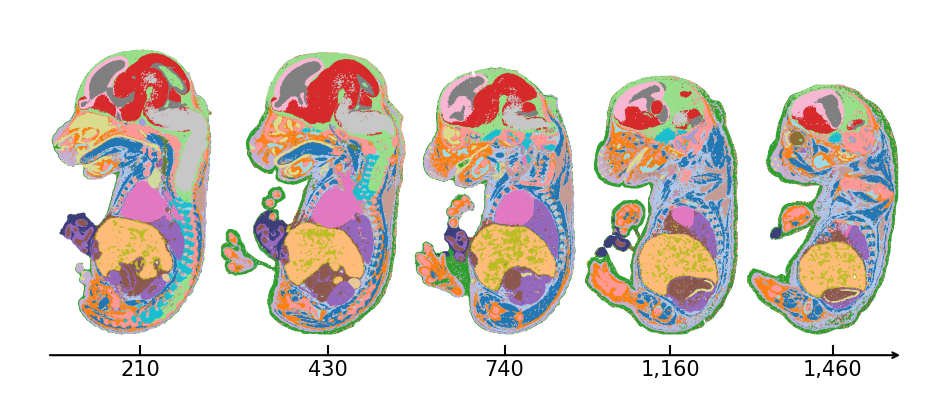
[16]:
loc_list = []
n_slices = len(set(adata_full.obs["slice_label"]))

for i in range(n_slices):
    # Load data
    ad_tmp = adata[adata.obs["slice_label"].values.astype(str) == str(i), :]
    loc_list.append(ad_tmp.obsm["spatial"])

size = 0.5

# louvain
f = plt.figure(figsize=(12,5))
ax = f.add_subplot(1,1,1)
ax.axis('equal')
colors = rgb2hex
for i in range(n_louvain):
    ax.scatter(adata.obsm["spatial"][adata.obs["anno"].values.astype(str)==str(i), 0],
               -adata.obsm["spatial"][adata.obs["anno"].values.astype(str)==str(i), 1],
               s=size, facecolors=colors[i], edgecolors='none', label="cluster "+str(i), rasterized=True)

y_arrow = -600
e_val_list = ["210","430","740","1,160","1,460"]

ax.annotate("", xy=(max(loc_list[-1][:,0])+10, y_arrow), xytext=(min(loc_list[0][:,0])-10, y_arrow), arrowprops=dict(arrowstyle="->", lw=1.5))
for i in range(len(loc_list)):
    x_m = np.median(loc_list[i][:, 0])
    plt.vlines(x = x_m, ymin=y_arrow, ymax=y_arrow+20, color = 'k')
    e_val = e_val_list[i]
    plt.annotate(e_val, xy=(x_m, y_arrow-40), ha='center', fontsize=15)

ax.set_axis_off()
plt.show()
Save results
[17]:
res_path = "Results/INSPIRE_3d_reconstruction"
adata_full.write(res_path + "/adata_inspire.h5ad")
basis_df.to_csv(res_path + "/basis_df_inspire.csv")
[ ]: