Run INSPIRE on the whole-embryo datasets generated by seqFISH and Stereo-seq
In this tutorial, we show INSPIRE’s capability of integrating and interpreting ST whole-embryo datasets across different technologies (seqFISH and Stereo-seq). The cross-technology integration enables multiple downstream analysis to facilitate deep biological insights.
The mouse whole-embryo slice profiled by seqFISH is publicly available at https://crukci.shinyapps.io/SpatialMouseAtlas/.
The mouse whole-embryo slice profiled by Stereo-seq is publicly available at https://db.cngb.org/stomics/mosta/.
Import packages
[1]:
import pandas as pd
import numpy as np
import scanpy as sc
import anndata as ad
import umap
import os
import matplotlib.pyplot as plt
import matplotlib as mpl
from matplotlib.cm import get_cmap
from matplotlib.lines import Line2D

import INSPIRE

import warnings
warnings.filterwarnings("ignore")
Load data
[2]:
print("Load seqFISH data...")

data_dir = "data/seqFISH_mouse_embryo"
counts = pd.read_csv(data_dir+"/counts.csv", index_col=0)
metadata = pd.read_csv(data_dir+"/metadata.csv", index_col=0)
metadata = metadata.loc[counts.index, :]
adata_seqfish = ad.AnnData(np.array(counts.values))
adata_seqfish.var.index = counts.columns
adata_seqfish.obs = metadata

adata_seqfish = adata_seqfish[adata_seqfish.obs["embryo"] == "embryo2", ]
adata_seqfish = adata_seqfish[adata_seqfish.obs["celltype_mapped_refined"] != "Low quality", ]
adata_seqfish.obsm["spatial"] = np.array(adata_seqfish.obs[["x_global", "y_global"]])
adata_seqfish.var_names_make_unique()
Load seqFISH data...
[3]:
print("Load Stereo-seq data...")

data_dir = "data/Stereoseq_mouse_embryo"
adata_stereoseq = sc.read_h5ad(os.path.join(data_dir, "E9.5_E1S1.MOSTA.h5ad"))
adata_stereoseq.X = adata_stereoseq.layers['count']
adata_stereoseq.var_names_make_unique()
Load Stereo-seq data...
[4]:
adata_st_list = [adata_seqfish, adata_stereoseq]
Data preprocessing
[5]:
adata_st_list, adata_full = INSPIRE.utils.preprocess(adata_st_list=adata_st_list,
                                                     num_hvgs=1000,
                                                     min_genes_qc=2,
                                                     min_cells_qc=2,
                                                     spot_size=1,
                                                     limit_num_genes=True)
Get shared genes among all datasets...
Find 347 shared genes among datasets.
Finding highly variable genes...
shape of adata 0 before quality control:  (14185, 347)
shape of adata 0 after quality control:  (14185, 347)
shape of adata 1 before quality control:  (5913, 347)
shape of adata 1 after quality control:  (5880, 344)
Find 344 shared highly variable genes among datasets.
Concatenate datasets as a full anndata for better visualization...

Store counts and library sizes for Poisson modeling...
Normalize data...
Build spatial graph and prepare node features for LGCN
[6]:
adata_st_list = INSPIRE.utils.build_graph_LGCN(adata_st_list=adata_st_list,
                                               rad_cutoff_list=[3,1.6])
Start building graphs...
Build graphs and prepare node features for LGCN networks
Radius for graph connection is 3.0000.
26.7748 neighbors per cell on average.
Node features for slice 0 : (14185, 688)
Radius for graph connection is 1.6000.
7.7946 neighbors per cell on average.
Node features for slice 1 : (5880, 688)
Run INSPIRE model
[8]:
model = INSPIRE.model.Model_LGCN(adata_st_list=adata_st_list,
                                 n_spatial_factors=40,
                                 n_training_steps=10000,
                                 batch_size=2048,
                                 different_platforms=True
                                 )
[9]:
model.train(adata_st_list)
0%| | 6/10000 [00:00<07:48, 21.34it/s]
Step: 0, d_loss: 1.4992, Loss: 1364.8623, recon_loss: 552.5065, fe_loss: 44.9286, geom_loss: 165.7725, beta_loss: 763.3344, gan_loss: 0.7776
5%|▌ | 506/10000 [00:11<03:29, 45.35it/s]
Step: 500, d_loss: 0.6237, Loss: 1167.3342, recon_loss: 433.0272, fe_loss: 28.1169, geom_loss: 87.4508, beta_loss: 702.1931, gan_loss: 2.2480
10%|█ | 1006/10000 [00:22<03:16, 45.76it/s]
Step: 1000, d_loss: 0.3045, Loss: 1076.6626, recon_loss: 341.4729, fe_loss: 27.3702, geom_loss: 130.6975, beta_loss: 701.8184, gan_loss: 3.3872
15%|█▌ | 1506/10000 [00:33<03:07, 45.34it/s]
Step: 1500, d_loss: 0.2098, Loss: 1014.6364, recon_loss: 279.4295, fe_loss: 26.9022, geom_loss: 131.7953, beta_loss: 701.8845, gan_loss: 3.7844
20%|██ | 2006/10000 [00:44<02:56, 45.35it/s]
Step: 2000, d_loss: 0.2105, Loss: 973.4398, recon_loss: 237.6814, fe_loss: 26.6580, geom_loss: 124.8234, beta_loss: 702.2662, gan_loss: 4.3377
25%|██▌ | 2506/10000 [00:55<02:43, 45.73it/s]
Step: 2500, d_loss: 0.2238, Loss: 949.7872, recon_loss: 214.8734, fe_loss: 26.5242, geom_loss: 119.8150, beta_loss: 702.2215, gan_loss: 3.7718
30%|███ | 3006/10000 [01:06<02:33, 45.69it/s]
Step: 3000, d_loss: 0.1744, Loss: 928.3311, recon_loss: 194.4388, fe_loss: 26.3288, geom_loss: 109.8261, beta_loss: 701.8584, gan_loss: 3.5087
35%|███▌ | 3506/10000 [01:17<02:22, 45.62it/s]
Step: 3500, d_loss: 0.1483, Loss: 922.0637, recon_loss: 187.6211, fe_loss: 26.2629, geom_loss: 105.1442, beta_loss: 701.8630, gan_loss: 4.2138
40%|████ | 4006/10000 [01:28<02:12, 45.36it/s]
Step: 4000, d_loss: 0.2480, Loss: 909.9057, recon_loss: 176.3834, fe_loss: 26.1227, geom_loss: 100.0805, beta_loss: 701.8671, gan_loss: 3.5309
45%|████▌ | 4506/10000 [01:39<02:00, 45.52it/s]
Step: 4500, d_loss: 0.2300, Loss: 910.6376, recon_loss: 177.2427, fe_loss: 26.1271, geom_loss: 98.9051, beta_loss: 701.7460, gan_loss: 3.5437
50%|█████ | 5006/10000 [01:50<01:50, 45.24it/s]
Step: 5000, d_loss: 0.3022, Loss: 901.6885, recon_loss: 167.7816, fe_loss: 26.0828, geom_loss: 99.3437, beta_loss: 701.8264, gan_loss: 4.0109
55%|█████▌ | 5506/10000 [02:01<01:39, 45.32it/s]
Step: 5500, d_loss: 0.2461, Loss: 903.7646, recon_loss: 170.3498, fe_loss: 26.1392, geom_loss: 91.4499, beta_loss: 701.7339, gan_loss: 3.7127
60%|██████ | 6006/10000 [02:12<01:27, 45.77it/s]
Step: 6000, d_loss: 0.2192, Loss: 896.4146, recon_loss: 163.2331, fe_loss: 26.1898, geom_loss: 88.4344, beta_loss: 701.5472, gan_loss: 3.6757
65%|██████▌ | 6506/10000 [02:23<01:16, 45.75it/s]
Step: 6500, d_loss: 0.2820, Loss: 899.3956, recon_loss: 166.6798, fe_loss: 26.2029, geom_loss: 80.5115, beta_loss: 701.5717, gan_loss: 3.3311
70%|███████ | 7006/10000 [02:34<01:05, 45.50it/s]
Step: 7000, d_loss: 0.2347, Loss: 890.3608, recon_loss: 158.0955, fe_loss: 26.1279, geom_loss: 76.1080, beta_loss: 701.5854, gan_loss: 3.0298
75%|███████▌ | 7506/10000 [02:45<00:54, 45.69it/s]
Step: 7500, d_loss: 0.2511, Loss: 889.9950, recon_loss: 157.2804, fe_loss: 26.1080, geom_loss: 72.4438, beta_loss: 701.7313, gan_loss: 3.4264
80%|████████ | 8006/10000 [02:55<00:44, 45.29it/s]
Step: 8000, d_loss: 0.2183, Loss: 889.2778, recon_loss: 156.7681, fe_loss: 26.1152, geom_loss: 71.1025, beta_loss: 701.6929, gan_loss: 3.2796
85%|████████▌ | 8506/10000 [03:06<00:33, 45.12it/s]
Step: 8500, d_loss: 0.2201, Loss: 883.6912, recon_loss: 151.7068, fe_loss: 26.0463, geom_loss: 66.4949, beta_loss: 701.5209, gan_loss: 3.0872
90%|█████████ | 9006/10000 [03:18<00:22, 44.91it/s]
Step: 9000, d_loss: 0.2291, Loss: 884.2099, recon_loss: 151.7741, fe_loss: 26.0731, geom_loss: 65.6530, beta_loss: 701.6666, gan_loss: 3.3829
95%|█████████▌| 9506/10000 [03:29<00:10, 45.38it/s]
Step: 9500, d_loss: 0.2348, Loss: 883.2949, recon_loss: 151.3600, fe_loss: 26.0523, geom_loss: 62.8923, beta_loss: 701.4165, gan_loss: 3.2083
100%|██████████| 10000/10000 [03:39<00:00, 45.46it/s]
Access spot representations, proportions of spatial factors in spots, and gene loading matrix
[10]:
adata_full, basis_df = model.eval(adata_st_list, adata_full)
basis = np.array(basis_df.values)
Add cell/spot proportions of spatial factors into adata_full.obs...
Add cell/spot latent representations into adata_full.obsm['latent']...
Gene loading matrix is saved as basis.
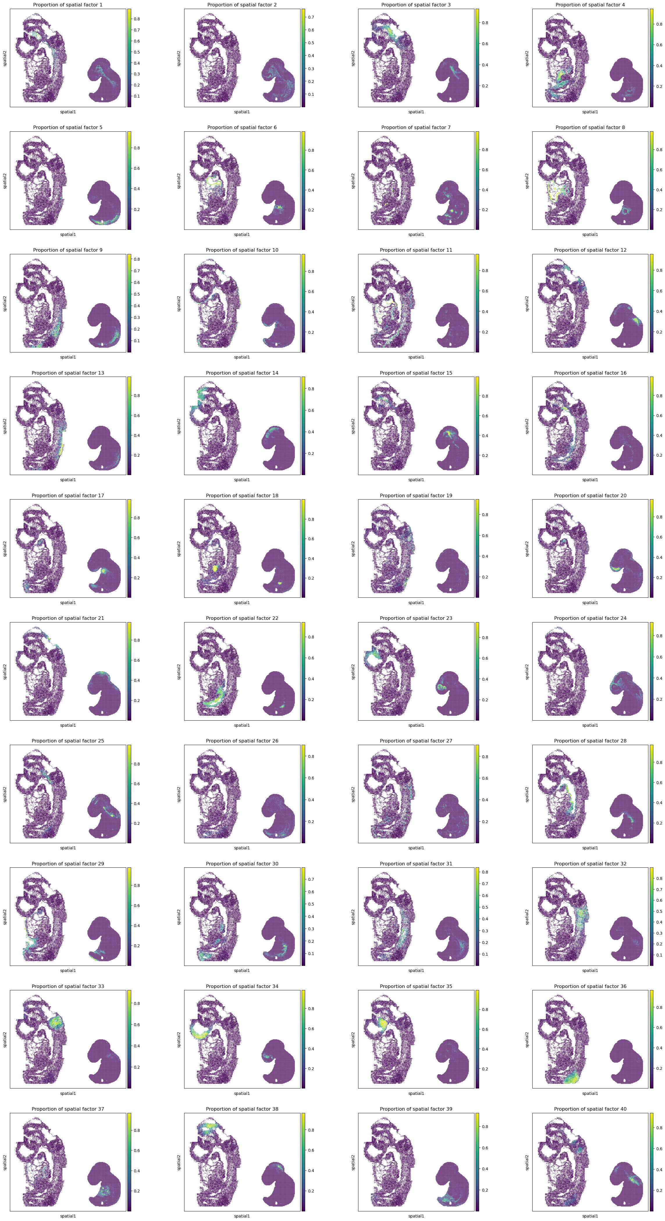
Spatial distributions of spatial factors in embryos
[11]:
sc.pl.spatial(adata_full, color=["Proportion of spatial factor "+str(i+1) for i in range(40)], spot_size=1.)
Spot representations and spatial domain identification
Calculate 2D UMAP coordinates of cells based on cell representations.
[12]:
reducer = umap.UMAP(n_neighbors=30,
                    n_components=2,
                    metric="correlation",
                    n_epochs=None,
                    learning_rate=1.0,
                    min_dist=0.3,
                    spread=1.0,
                    set_op_mix_ratio=1.0,
                    local_connectivity=1,
                    repulsion_strength=1,
                    negative_sample_rate=5,
                    a=None,
                    b=None,
                    random_state=1234,
                    metric_kwds=None,
                    angular_rp_forest=False,
                    verbose=True)
embedding = reducer.fit_transform(adata_full.obsm['latent'])
adata_full.obsm["X_umap"] = embedding
adata_full.obs["slice"] = adata_full.obs["slice"].values.astype(str)
UMAP(angular_rp_forest=True, local_connectivity=1, metric='correlation', min_dist=0.3, n_neighbors=30, random_state=1234, repulsion_strength=1, verbose=True)
Fri Aug 23 16:36:33 2024 Construct fuzzy simplicial set
Fri Aug 23 16:36:33 2024 Finding Nearest Neighbors
Fri Aug 23 16:36:33 2024 Building RP forest with 12 trees
Fri Aug 23 16:36:37 2024 NN descent for 14 iterations
         1  /  14
         2  /  14
         3  /  14
        Stopping threshold met -- exiting after 3 iterations
Fri Aug 23 16:36:45 2024 Finished Nearest Neighbor Search
Fri Aug 23 16:36:47 2024 Construct embedding
        completed  0  /  200 epochs
        completed  20  /  200 epochs
        completed  40  /  200 epochs
        completed  60  /  200 epochs
        completed  80  /  200 epochs
        completed  100  /  200 epochs
        completed  120  /  200 epochs
        completed  140  /  200 epochs
        completed  160  /  200 epochs
        completed  180  /  200 epochs
Fri Aug 23 16:37:07 2024 Finished embedding
Perform spatial domain identification jointly for the two slices by clustering the integrated cell representations.
[13]:
sc.pp.neighbors(adata_full, use_rep="latent", n_neighbors=30)
sc.tl.louvain(adata_full, resolution=.7)
Visualization of cell representations.
[14]:
adata = adata_full

size = 0.04
umap = adata.obsm["X_umap"]
n_cells = umap.shape[0]
np.random.seed(1234)
order = np.arange(n_cells)
np.random.shuffle(order)

adata.obs["slice_color"] = ""
adata.obs["slice_color"][adata.obs["slice"].values.astype(str) == str(0)] = "#A58AFF"
adata.obs["slice_color"][adata.obs["slice"].values.astype(str) == str(1)] = "#00C094"

f = plt.figure(figsize=(5,5))

ax3 = f.add_subplot(1,1,1)
scatter2 = ax3.scatter(umap[order, 0], umap[order, 1], s=size, c=adata.obs["slice_color"][order], rasterized=True, marker='o')
ax3.tick_params(axis='both',bottom=False, top=False, left=False, right=False, labelleft=False, labelbottom=False, grid_alpha=0)

legend_elements_slice = [Line2D([0], [0], marker='o', color="w", label='seqFISH', markerfacecolor="#A58AFF", markersize=10),
                         Line2D([0], [0], marker='o', color="w", label='Stereo-seq', markerfacecolor="#00C094", markersize=10)]
ax3.legend(handles=legend_elements_slice, loc="upper left", bbox_to_anchor=(1, 1), frameon=False,
           markerscale=.8, fontsize=10, handletextpad=0., ncol=1)

f.subplots_adjust(hspace=0.02, wspace=0.1)
plt.show()

[15]:
# setup colors
rgb_10 = [i for i in get_cmap('Set3').colors]
rgb_20 = [i for i in get_cmap('tab20').colors]
rgb_20b = [i for i in get_cmap('tab20b').colors]
rgb_dark2 = [i for i in get_cmap('Dark2').colors]
rgb_pst1 = [i for i in get_cmap('Pastel1').colors]
rgb_acc = [i for i in get_cmap('Accent').colors]
rgb2hex_10 = [mpl.colors.rgb2hex(color) for color in rgb_10]
rgb2hex_20 = [mpl.colors.rgb2hex(color) for color in rgb_20]
rgb2hex_20b = [mpl.colors.rgb2hex(color) for color in rgb_20b]
rgb2hex_20b_new = [rgb2hex_20b[i] for i in [0, 3, 4, 7, 8, 11, 12, 15, 16, 19]]
rgb2hex_dark2 = [mpl.colors.rgb2hex(color) for color in rgb_dark2]
rgb2hex_pst1 = [mpl.colors.rgb2hex(color) for color in rgb_pst1]
rgb2hex_acc = [mpl.colors.rgb2hex(color) for color in rgb_acc]
rgb2hex = rgb2hex_20 + rgb2hex_20b_new + rgb2hex_dark2 + rgb2hex_pst1 + rgb2hex_acc
colors = rgb2hex
adata.obs["louvain_color"] = ""
for i in range(len(set(adata.obs["louvain"].values.astype(str)))):
    adata.obs["louvain_color"][adata.obs["louvain"].values.astype(str) == str(i)] = colors[i]

adata.obs["louvain_color"][adata.obs["louvain"].values.astype(str) == str(1)] = rgb2hex[13]
adata.obs["louvain_color"][adata.obs["louvain"].values.astype(str) == str(13)] = rgb2hex[1]

adata.obs["louvain_color"][adata.obs["louvain"].values.astype(str) == str(4)] = rgb2hex[6]
adata.obs["louvain_color"][adata.obs["louvain"].values.astype(str) == str(6)] = rgb2hex[15]
adata.obs["louvain_color"][adata.obs["louvain"].values.astype(str) == str(15)] = rgb2hex[4]
[16]:
size = 0.04
umap = adata.obsm["X_umap"]
n_cells = umap.shape[0]
np.random.seed(1234)
order = np.arange(n_cells)
np.random.shuffle(order)

f = plt.figure(figsize=(5,5))

ax3 = f.add_subplot(1,1,1)
scatter2 = ax3.scatter(umap[order, 0], umap[order, 1], s=size, c=adata.obs["louvain_color"][order], rasterized=True, marker='o')
ax3.tick_params(axis='both',bottom=False, top=False, left=False, right=False, labelleft=False, labelbottom=False, grid_alpha=0)

for i in range(len(set(adata.obs["louvain"].values.astype(str)))):
    coor_tmp = umap[adata.obs["louvain"].values.astype(str) == str(i), :]
    coor_xy = np.median(coor_tmp, axis=0)
    ax3.annotate(str(i), coor_xy)

f.subplots_adjust(hspace=0.02, wspace=0.1)
plt.show()

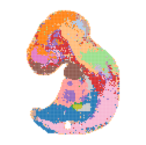
Visualization of spatial region identification result.
[17]:
size = 3

# louvain
f = plt.figure(figsize=(5,5))
ax = f.add_subplot(1,1,1)
ax.axis('equal')
colors = rgb2hex
adata_tmp = adata[adata.obs["slice"].values.astype(str) == "0", :]
ax.scatter(adata_tmp.obsm["spatial"][:, 0],
           -adata_tmp.obsm["spatial"][:, 1],
           s=size, facecolors=adata_tmp.obs["louvain_color"], edgecolors='none', rasterized=True)
ax.set_axis_off()
f.subplots_adjust(hspace=0.02, wspace=0.1)
plt.show()

[18]:
size = 4

# louvain
f = plt.figure(figsize=(3.5,3.5))
ax = f.add_subplot(1,1,1)
ax.axis('equal')
colors = rgb2hex
adata_tmp = adata[adata.obs["slice"].values.astype(str) == "1", :]
ax.scatter(adata_tmp.obsm["spatial"][:, 0],
           -adata_tmp.obsm["spatial"][:, 1],
           s=size, facecolors=adata_tmp.obs["louvain_color"], edgecolors='none', rasterized=True)
ax.set_axis_off()
f.subplots_adjust(hspace=0.02, wspace=0.1)
plt.show()
Save results
[19]:
### Save results
res_path = "Results/INSPIRE_diff_tech_embryo"
adata_full.write(res_path + "/adata_inspire.h5ad")
basis_df.to_csv(res_path + "/basis_df_inspire.csv")
[ ]: